
Machine learning paradigms and mathematical foundations
Types of machine learning, common algorithms and essential mathematical foundations for understanding how machine learning models work.
We continue learning about Machine Learning, this time we will delve into the different paradigms of machine learning and the mathematical foundations that support these models.
Previous article: Machine Learning Fundamentals
Machine Learning Paradigms
In the previous article, we already mentioned the types of machine learning, in this section we will review them and then move on to the mathematical foundations.
Supervised Learning
Supervised learning requires a dataset where each input example X is associated with a label or output Y. The objective of the model is to learn a function that maps inputs to correct outputs.
Based on this, the training dataset is represented as a set of pairs , where is the input and is the corresponding label. The supervised learning model attempts to find a function f that can predict the output Y from the input X:
Depending on the type of output, supervised learning can be divided into:
- Classification: When the output Y is a discrete category (that is, a categorical value). For example, classifying whether an image contains a cat or a dog, whether a number is even or odd, or whether an email is spam or not spam.
- Regression: When the output Y is a continuous value (that is, a real number). For example, making predictions about future sales based on historical data, predicting the price of a house based on its features, or estimating the temperature of a city based on climatic factors.
Unsupervised Learning
In unsupervised learning, the model receives only the inputs X without associated labels: . The objective is to find underlying patterns or structures in the data. Some examples of unsupervised learning techniques include:
- Clustering: Grouping similar data points into clusters. For example, segmenting customers into groups based on their purchasing behaviors.
- Dimensionality Reduction: Reducing the number of variables in a dataset while preserving as much information as possible. For example, using PCA (Principal Component Analysis) to visualize data in 2D or 3D.
Reinforcement Learning
Reinforcement learning is based on the idea that an agent learns to make decisions by interacting with an environment. The agent receives rewards or penalties based on the actions it takes, and its objective is to maximize the accumulated reward over time. In this paradigm, the agent learns an action policy that allows it to make optimal decisions based on the current state of the environment. A classic example of reinforcement learning is the game of chess, where the agent learns to play better as it plays more games and receives feedback about its moves.
- Agent: The system that makes decisions.
- Environment: The world with which the agent interacts.
- Reward: The feedback that the agent receives after taking an action.
- Policy: The strategy that the agent follows to make decisions.
Its applications include games, robotics, and recommendation systems.
Mathematical Foundations
It is important to understand that machine learning is based on concepts from linear algebra, calculus, probability, and statistics. These fundamentals are essential for understanding how models work and how they are optimized.
Regression
What is a regression problem? It is a type of problem where the objective is to predict a continuous value by finding the best line (or plane) that fits the data. We have already discussed application examples such as price calculation, sales forecasting, etc.
The simplest form of regression is linear regression, which can be mathematically expressed as:
Where:
- is the dependent variable (what we want to predict).
- are the independent variables (the features).
- is the intercept (the value of when all are 0).
- are the coefficients that represent the influence of each feature on the dependent variable.
- is the error or noise value, which represents the variability not explained by the model, that is, what affects but is not included in the independent variables.
The objective of the regression model is to find the values of the coefficients that minimize the difference between the model's predictions and the real values of . This can be achieved using techniques such as the least squares method.
The intercept is represented as the first element of the coefficient vector , and it is the value of when all the independent variables in are zero, that is, it represents the point where the regression line crosses the Y-axis.
The slope is represented by the remaining coefficients in the vector , and each coefficient indicates the amount of change in the dependent variable for each unit change in the corresponding independent variable in , keeping all other independent variables constant. Graphically we can see it as follows:
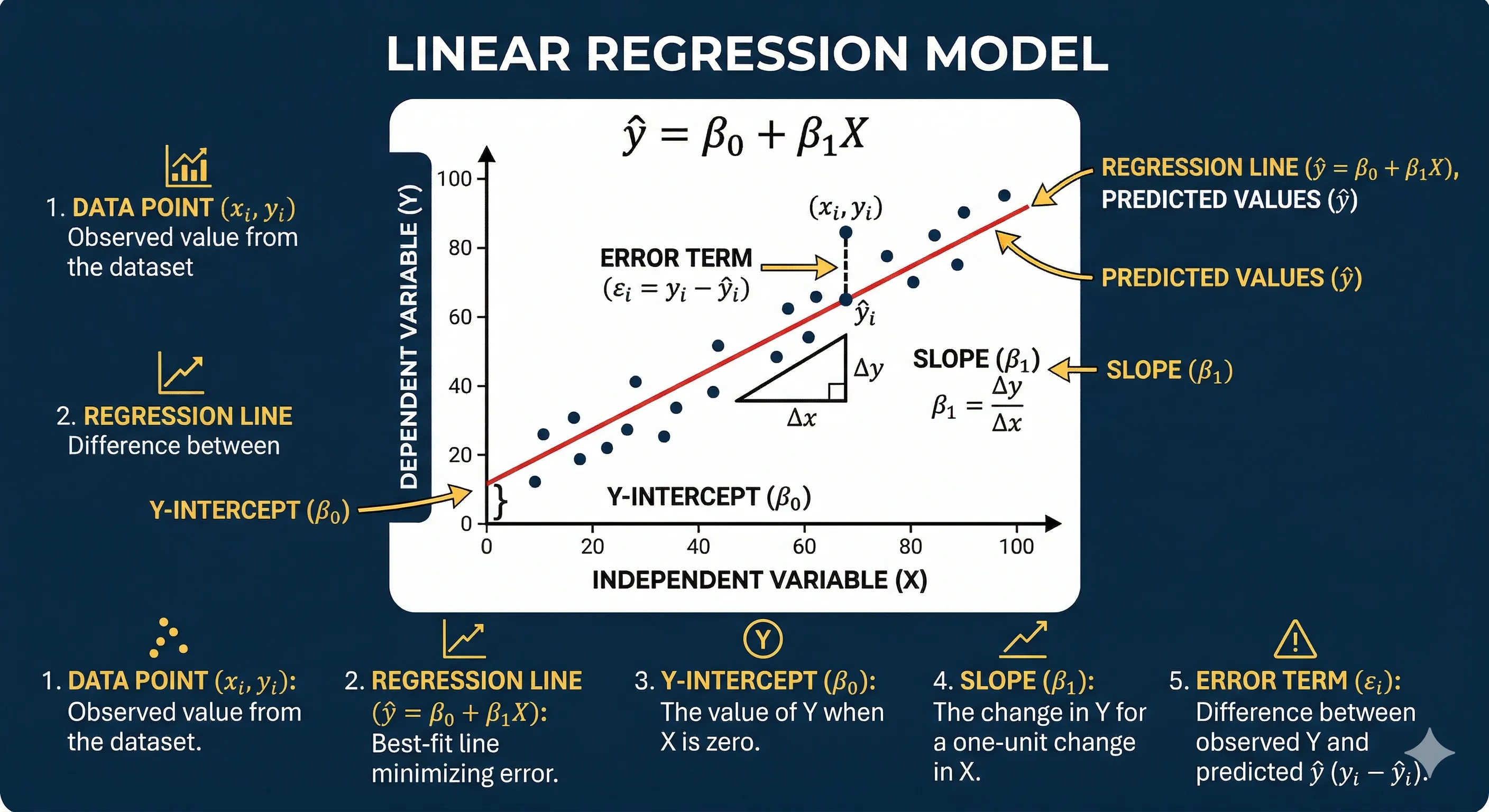 Linear Regression Graph
Each black point represents a training data point, and the red line represents the model.
The key point here is to understand that the main objective is to find the values of the coefficients that make the predictions (the red line) as close as possible to the actual values.
That is, we do not seek to predict with perfect accuracy, as (in reality) there will always be some error or difference between what the model predicts and what actually happens. The term is the difference between the values predicted by the model and the actual values:
Which can also be expressed as:
To measure the error we can use a loss function. In the case of linear regression, a commonly used loss function is the mean squared error (MSE, for its acronym in English), which is defined as:
Where:
- is the number of examples in the dataset.
- is the actual value of the dependent variable for example .
- is the model's prediction for example .
Minimizing the MSE is equivalent to minimizing the sum of squared errors:
Or also:
This is known as the least squares method, and it is a commonly used technique to find the coefficients that best fit the data.
Why are squares used? Because by squaring the differences, larger errors are penalized more, which helps to find a better fitting line for the data.
Let's now see how we obtain those coefficients using the least squares method. To find the values of and , we can use the following formulas, which are obtained by taking the derivative of the MSE loss function with respect to the coefficients and setting the derivatives equal to zero:
Where:
- is the number of examples in the dataset.
- and are the values of the independent and dependent variables for each example.
- and are the means (or averages) of the independent and dependent variables, respectively.
Let's do an example to understand how to apply it. Suppose we have a dataset with the following characteristics:
| Size (m²) | Price (USD) |
|---|---|
| 50 | 100,000 |
| 100 | 200,000 |
| 150 | 300,000 |
We want to build a linear regression model to predict the price of a house based on its size. In this case, the independent variable is the size (X) and the dependent variable is the price (Y). The linear regression model can be expressed as:
Where:
- is the price of the house.
- is the size of the house.
- is the y-intercept.
- is the slope.
- is the error or noise, which for this example we will assume is zero for simplicity.
To find the values of and , we can use the least squares method with the formula we mentioned earlier:
Where:
- is the number of examples (in this case, 3).
- and are the values of size and price for each example.
- and are the means of the independent and dependent variables, respectively.
We have then for this case:
Solving these formulas, we obtain the values of and , which allow us to build the following model:
We can now make predictions for new size values. For example, for a 120 m² house, the model predicts a price of:
Our calculations have yielded the best coefficients that minimize the mean squared error (but do not eliminate it completely). To measure the error of our model, we can calculate the MSE using the formula mentioned earlier:
Where:
- is the number of examples (in this case, 3).
- are the real values of price for each example.
- are the model predictions for each example, which are calculated using the linear regression model.
- We calculate the predictions for each example:
- For 50 m²:
- For 100 m²:
- For 150 m²:
- We calculate the errors for each example:
- Error for 50 m²:
- Error for 100 m²:
- Error for 150 m²:
- We square the errors and average them to obtain the MSE:
For this case, an MSE of 0 indicates that the model predicts the real values perfectly for this training dataset. Of course, in practice, real data will contain noise and will be even more variable, so the epsilon will not be zero.
To explore more with regression, you can use this Google Colab that contains a complete example of linear regression with Python: linear_regression
Classification
A classification problem aims to predict a categorical output variable based on a set of input variables. For example, predicting whether an email is spam or not spam based on its content, or determining whether an image contains a cat or a dog.
There are three main types of classification:
- Binary Classification: When there are two possible classes. For example, classifying whether a patient has a disease (yes/no).
- Multi-class Classification: When there are more than two possible classes. For example, classifying the type of flower (could be setosa, versicolor or virginica) based on its characteristics.
- Multi-label Classification: When each example can belong to multiple classes, such as classifying the labels of a news article (politics, economy, sports) where an article can belong to several categories.
The difference between multi-class and multi-label classification is that in the former each example can only belong to one class, while in the latter an example can belong to multiple classes simultaneously.
Let's look a bit more at binary classification. In this case, the objective is to find a function that maps the inputs to one of the two possible classes.
The question that the binary classification model attempts to answer is: What is the probability that an example belongs to class 1 given a set of features? This can be expressed mathematically as: Where:
- is the probability that the class is 1 given the feature vector x.
- is the function that maps the features to the probability.
The most common model for binary classification is the logistic regression, which has the following process:
- We calculate a linear combination of the features:
- We apply the sigmoid function to obtain a probability:
- Class probability:
Where:
- is the intercept.
- are the coefficients that represent the influence of each feature on the dependent variable.
- are the features or independent variables.
- is the probability that the class is 1 given the feature vector x.
Each feature provides evidence for or against a particular class. For example, if the word "free" appears in an email, it might increase the probability that it is spam. On the other hand, if the word "meeting" appears, it might decrease the probability of it being spam.
This gives us not only a classification but also a measure of confidence in that classification through the probability calculated by the sigmoid function.
The sigmoid function transforms any real value into a value between 0 and 1. The formula as shown above is:
Where:
- is the linear combination of the features, that is, .
- is Euler's number, approximately equal to 2.71828.
- is the output of the sigmoid function, which represents the probability of the class being 1 given the value of z (range between 0 and 1).
Visually it looks something like this (with z on the X-axis and on the Y-axis):
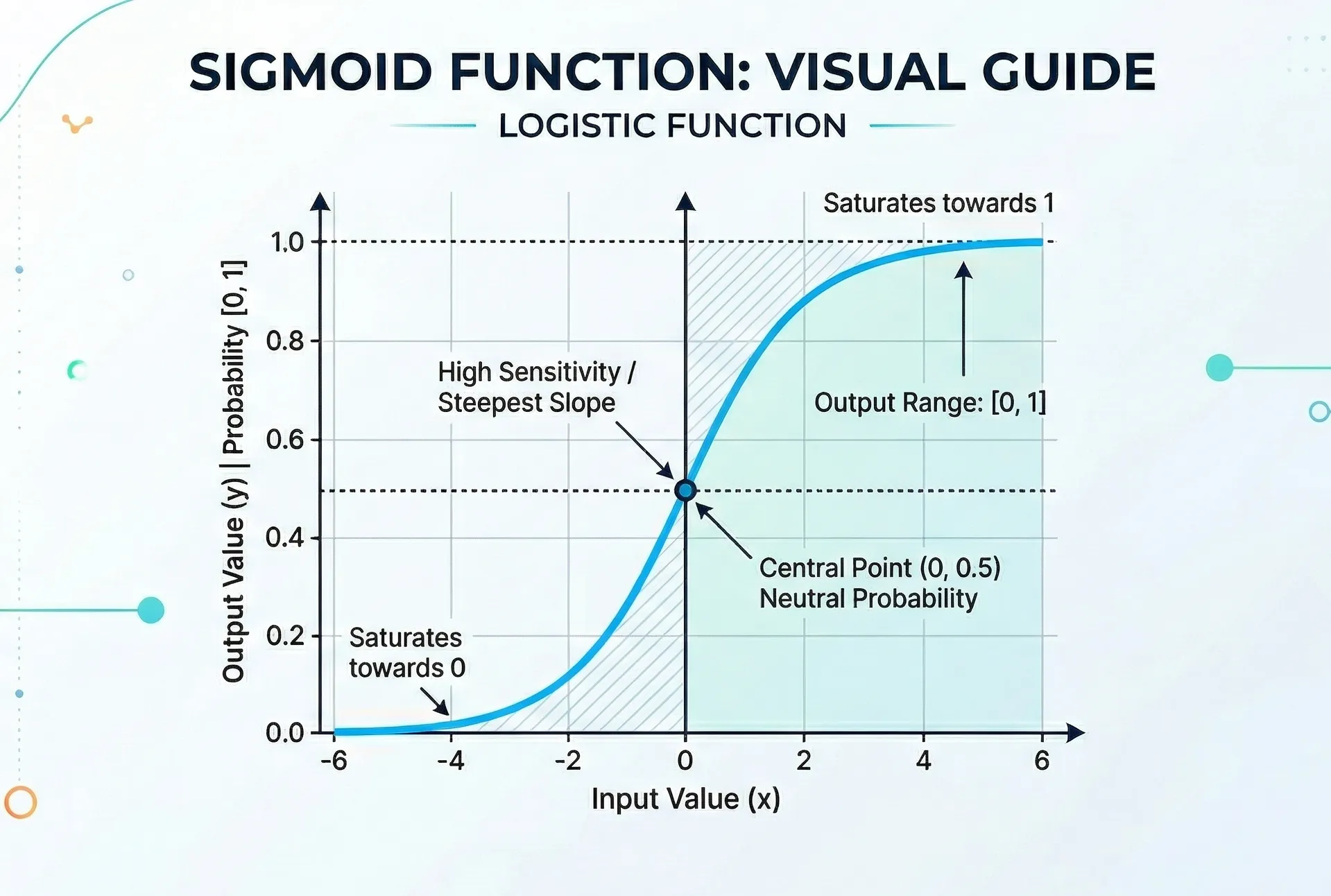 Sigmoid Function Graph
From this we can draw some important conclusions:
- When z is very negative, approaches 0, indicating a low probability that the class is 1.
- When z is very positive, approaches 1, indicating a high probability that the class is 1.
- When z is 0, is 0.5, indicating an equal probability that the class is 0 or 1.
The value of 0.5 is commonly used as a threshold, so that:
- If , it is classified as class 1.
- If , it is classified as class 0.
Key properties:
- Bounded range between 0 and 1
- Monotonicity: if z increases, also increases
- Asymptotic: when and when
How do we measure error in classification? Here we use metrics like cross-entropy or log loss:
Loss for a single sample:
Average loss (or cost function) for the entire dataset:
Where:
- is the number of examples in the dataset.
- is the true label (0 or 1) for example .
- is the predicted probability by the model for example (value between 0 and 1).
Why is cross-entropy used?
- It penalizes incorrect predictions with high confidence more heavily.
- It is a convex loss function, which makes optimization easier using methods like gradient descent.
- It has a probabilistic interpretation, as it is based on the predicted probability by the model.
The behavior of the loss function is shown in the following graph:
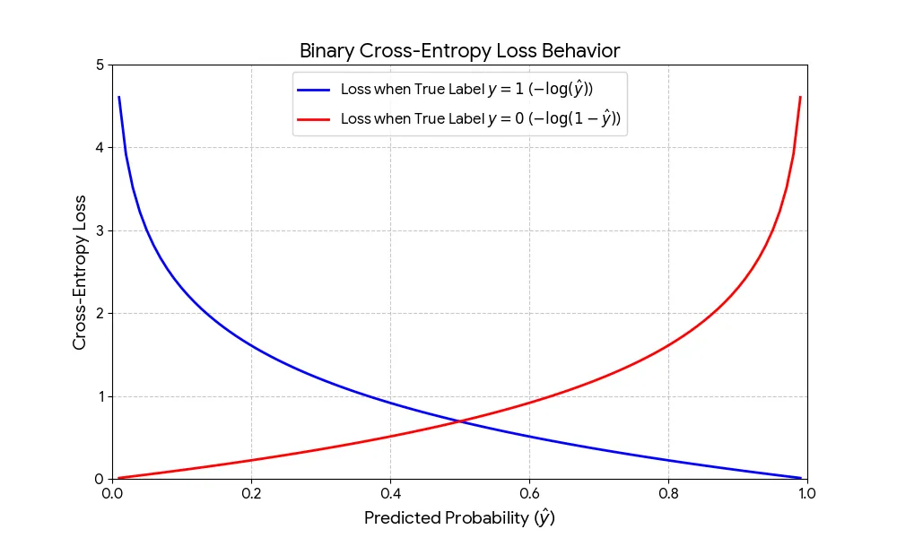 Cross-Entropy Loss Function Graph
The function penalizes more heavily the incorrect predictions with high confidence, which is reflected in the shape of the curve.
- When the true label is 1 (y=1) (blue line):
- The formula simplifies to
- If approaches 1, the loss approaches 0 (good prediction).
- If approaches 0, the loss shoots to infinity (bad prediction).
- When the true label is 0 (y=0) (red line):
- The formula simplifies to
- If approaches 0, the loss approaches 0 (good prediction).
- If approaches 1, the loss shoots to infinity (bad prediction).
The logarithmic nature of the function ensures that the model is heavily penalized when it is "confident but wrong", forcing it to adjust its weights more aggressively to improve predictions.
Validation and Optimization
Evaluation Metrics
For regression, the common metrics include:
- Mean Squared Error (MSE): Average of the squares of the differences between the actual values and the predictions.
- Root Mean Squared Error (RMSE): Square root of the MSE, which has the same unit as the dependent variable.
- Coefficient of Determination (R²): Proportion of the variance in the dependent variable that is explained by the model.
For classification, the common metrics include:
- Accuracy: Proportion of correct predictions over the total number of examples.
- Precision: Proportion of true positives over the total number of positive predictions.
- Recall (Sensitivity): Proportion of true positives over the total number of actual positive examples.
- F1 Score: Harmonic mean of precision and recall, providing a balanced measure between both.
The choice of the appropriate metric depends on the context of the problem and the consequences of classification errors. For example, in a fraud detection problem, it is more important to minimize false negatives (failing to detect fraud) than false positives (marking a legitimate transaction as fraud), so recall could be a more relevant metric than precision.
Optimization
Optimization of machine learning models refers to the process of adjusting the model parameters to minimize the loss function. This can be achieved through techniques like gradient descent, which iteratively adjusts the model weights in the direction that reduces the loss.
Gradient descent can be mathematically expressed as:
Where:
- represents the model parameters (for example, the coefficients in regression).
- is the learning rate, which controls the size of the steps taken in each iteration.
- is the gradient of the loss function with respect to the parameters, indicating the direction of greatest increase in the loss.
The optimization process continues until a convergence criterion is met, such as a maximum number of iterations or a minimum improvement in the loss function.
- It has a learning rate () that controls the size of the steps taken in each iteration (typically a small value like 0.01 or 0.001).
- The gradient () is a vector containing the partial derivatives of the loss function with respect to each parameter, indicating the direction of greatest increase in the loss.
- The optimization process continues until a convergence criterion is met, such as a maximum number of iterations or a minimum improvement in the loss function.
Graphically:
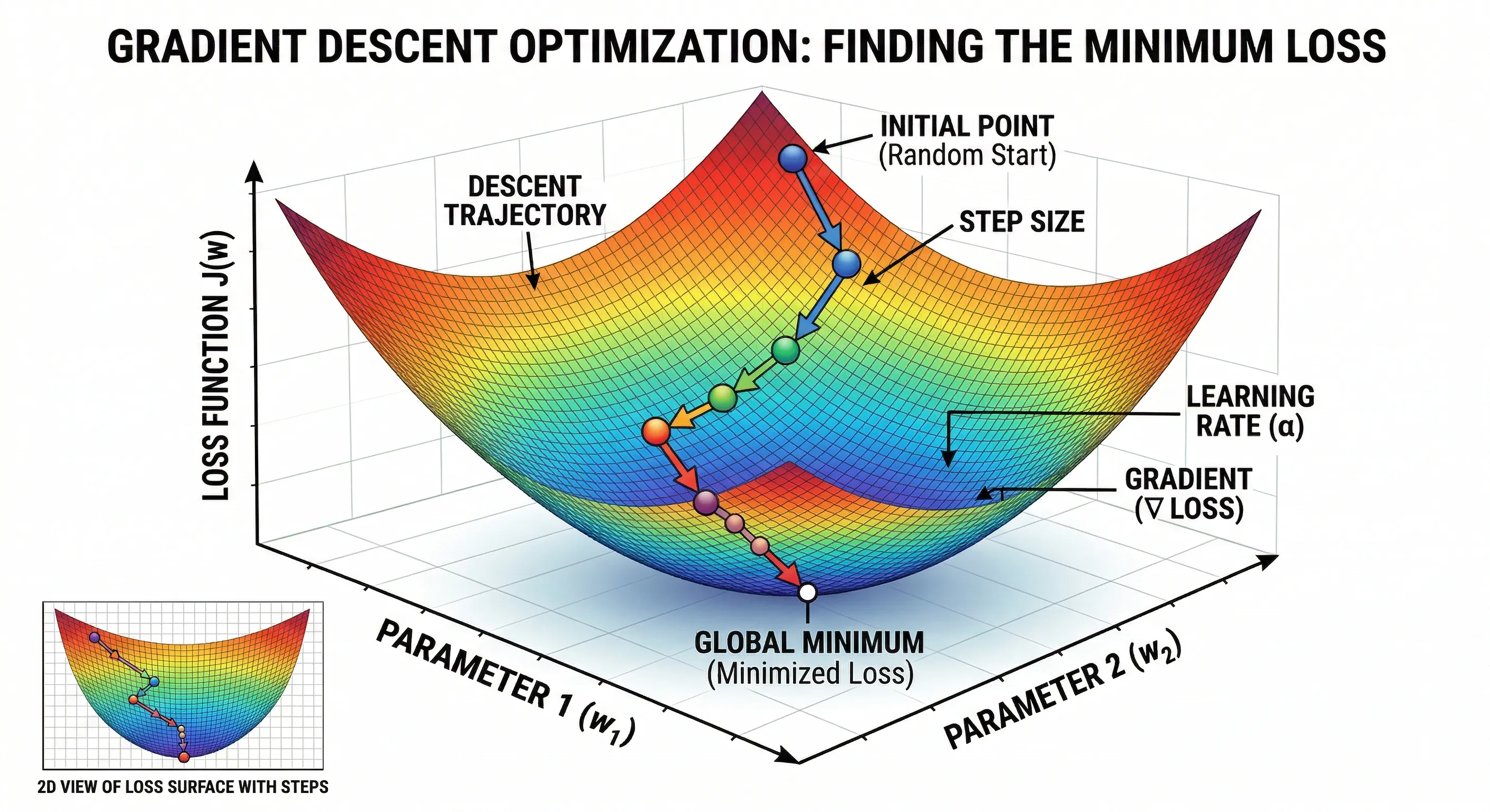 Optimization with Gradient Descent
- The process starts with a random point on the loss function (INITIAL POINT).
- The gradient is calculated at that point, indicating the direction of greatest increase in the loss.
- The model parameters are updated in the opposite direction of the gradient, with a step size controlled by the learning rate (LEARNING RATE / STEP SIZE).
- This process is repeated iteratively until a local or global minimum of the loss function is reached, indicating that the model has been optimized.
The learning rate is crucial for the success of the optimization process:
- DIVERGENCE: If the learning rate is too high, the model may diverge, jumping over the minimum and increasing the loss.
- SLOW CONVERGENCE: If the learning rate is too low, the optimization process may be very slow, taking a long time to converge or getting stuck in a local minimum.
- OPTIMAL CONVERGENCE: An appropriate learning rate allows the model to converge efficiently towards a global or local minimum, effectively optimizing the loss function.
The Machine Learning Process
We can summarize the ML process in:
- Learning Paradigm: Choose the type of learning (supervised, unsupervised, reinforcement) based on the problem to solve.
- Define the type of problem and available data.
- Mathematical Model: Select an appropriate model (regression, classification, clustering) and understand its mathematical formulation.
- Establish the mathematical relationship between input and output.
- Loss/Cost Function: Define a loss function that measures the model's error and can be optimized.
- Quantifies how bad the model is in its predictions.
- Optimization: Use techniques like gradient descent to adjust the model parameters and minimize the loss function.
- Finds the best parameters for the model to make good predictions.
- Evaluation: Measure the model's performance using appropriate metrics for the problem type (MSE for regression, accuracy/recall for classification, etc.).
- Validates the performance of the model and its ability to generalize to unseen data.