The workflow in Machine Learning projects
Discover the typical workflow of a machine learning project, from data collection to model implementation, and learn about best practices and common challenges in the field of data science.
We continue learning about the world of machine learning, and this time, we will delve into the typical flow of a machine learning project.
Previous article: Paradigms of machine learning and mathematical foundations
Why is it important to understand the workflow of a machine learning project?
- The process is more important than the result: Successful models do not depend solely on sophisticated algorithms, but on a well-structured process. A Random Forest with clean and well-prepared data consistently outperforms a deep neural network with poor-quality data.
- Reproducibility: A clear and documented workflow allows other data scientists to reproduce your results, which is fundamental for validation and advancing knowledge in the field.
- Collaboration: In machine learning projects, there are often multiple people involved, from data scientists to data engineers and stakeholders. A well-defined workflow facilitates communication and collaboration among all team members.
- Reduces the risk of errors: A structured process helps identify and correct errors in the early stages of the project, which can save time and resources in the long run.
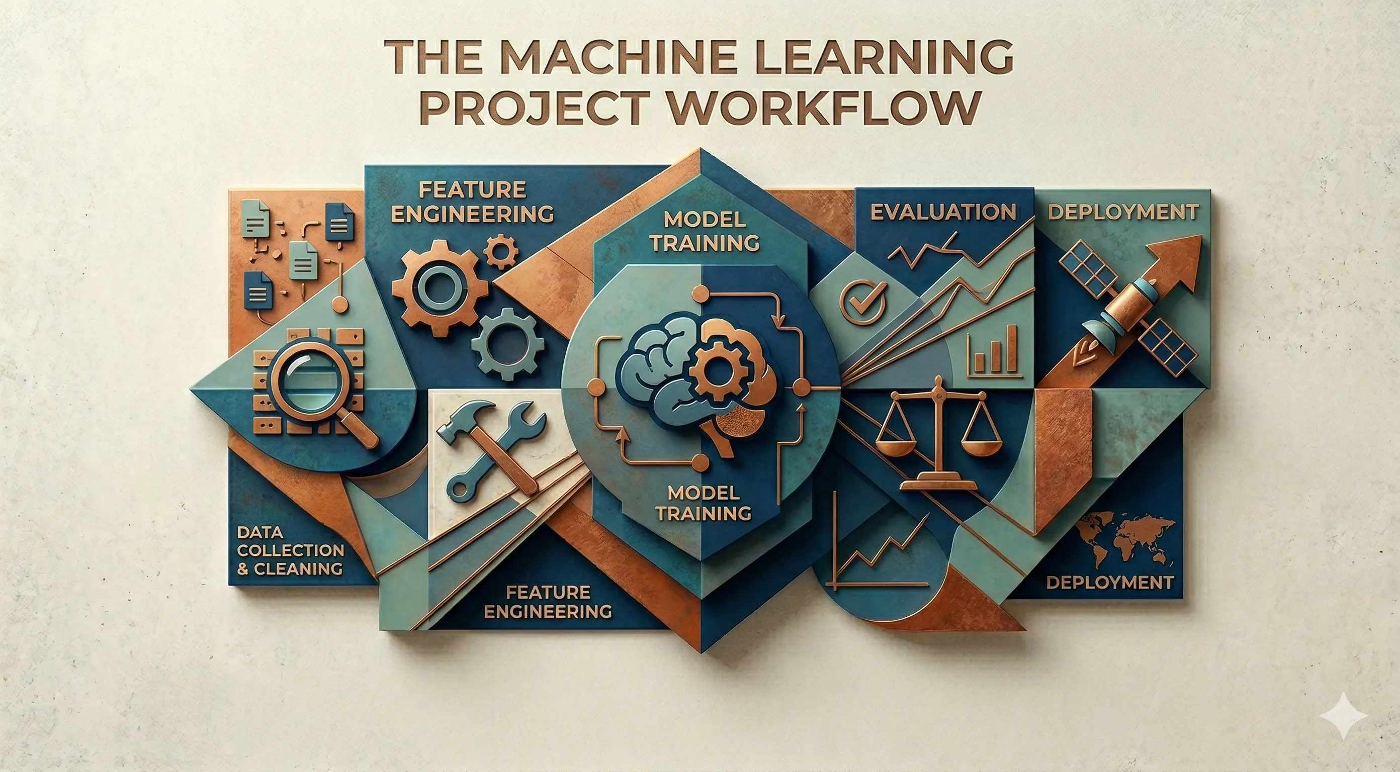
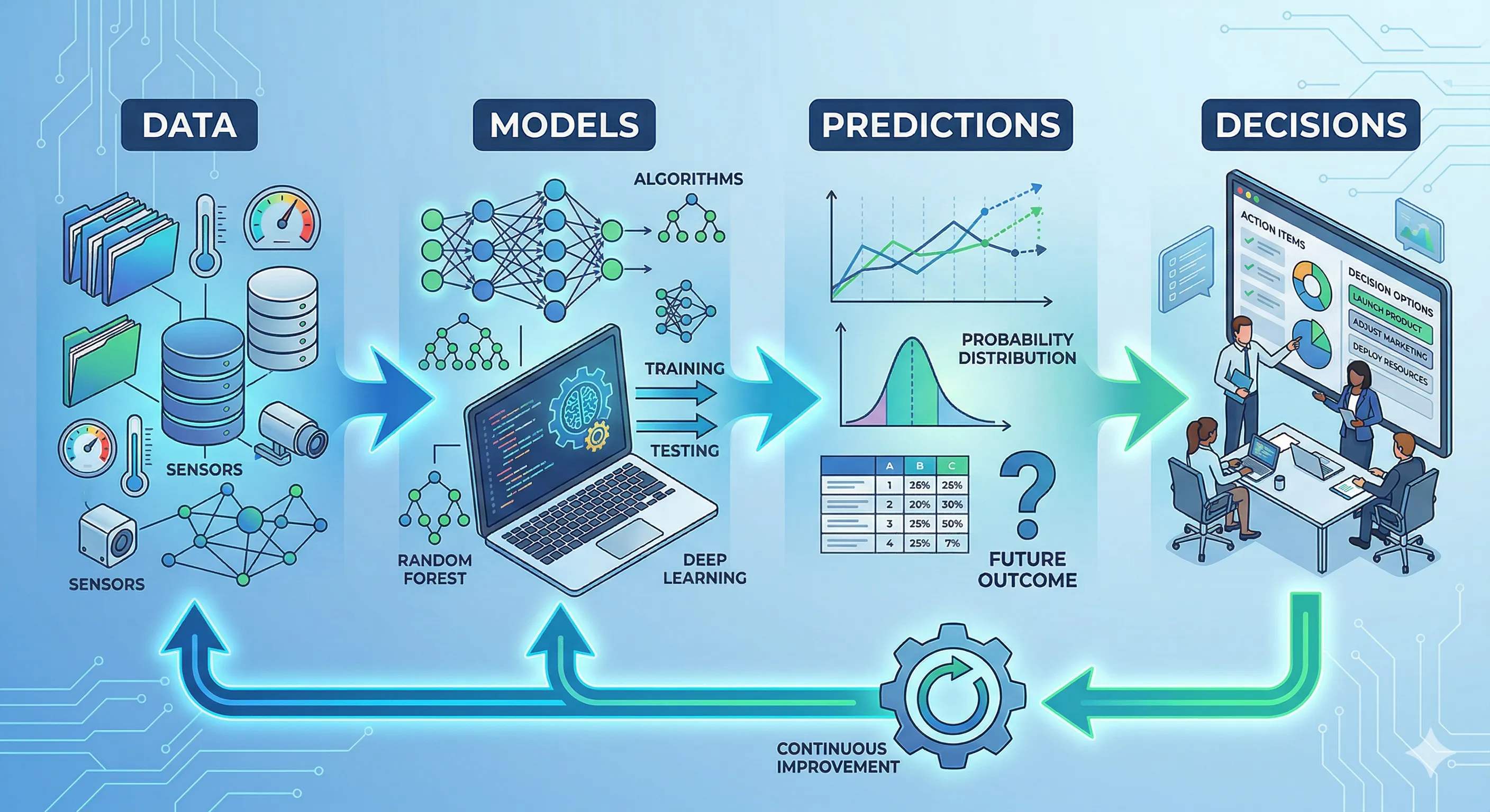
In general, machine learning is a process that is part of a system, with an iterative cycle and value-driven approach that consists of several stages, each with their own tasks and challenges.
 Machine Learning Cycle
1. Problem Definition
The first stage of any machine learning project is the problem definition:
- Problem Identification: What do we want to achieve with the project? What decisions do we want to support with the model? It is crucial to understand the business context or application to clearly define the problem.
- Target Variable: What is the variable we want to predict or classify? This variable, also known as the dependent variable, is the focus of the project and must be clearly defined.
- Type of Problem: Is it a classification, regression, clustering, or something else? The nature of the problem will influence the choice of algorithms and techniques to use.
- Evaluation Metrics: How will we measure the success of the model? It is important to define evaluation metrics from the beginning, as these will guide the model development and decision-making throughout the project.
This stage is the foundation of the entire project. A poorly defined problem can lead to wasted efforts and unsatisfactory results. It is fundamental to dedicate time to understanding the problem and setting clear objectives before moving on to subsequent stages.
Let's look at a practical example: Suppose an e-commerce company wants to predict whether a customer will make a purchase on their website. In this case:
- Problem Identification: Predicting the probability of a customer making a purchase.
- Target Variable: The target variable could be a binary variable indicating whether the customer made a purchase (1) or not (0).
- Type of Problem: This is a binary classification problem.
- Evaluation Metrics: The evaluation metrics could include accuracy, recall, and F1-score, depending on the relative importance of false positives and false negatives in the business context.
2. Data Collection
Once the problem is clearly defined, the next step is data collection, where relevant data sources must be identified and accessed. This can include:
- Internal/Enterprise Databases: Data stored in internal company systems, such as relational databases, data warehouses or data lakes. Some examples include sales records, customer data, data from CRM or ERP systems, among others.
- APIs and Web Services: External data from data providers, social media, geolocation services, etc. For example, a sentiment analysis company could use the Twitter API to collect tweets related to a specific topic.
- System Logs and Event Records: Data generated by applications, servers, IoT devices, etc. For example, an infrastructure monitoring company could collect server logs to detect failure patterns.
- Public/External Data: Data available publicly, such as datasets from Kaggle, government data, academic research data, etc. For example, a researcher could use the MNIST image dataset to train a handwritten digit recognition model.
It is important to note that the quality of the collected data is crucial for the success of the project. The data must be relevant, complete, accurate and up-to-date. Additionally, it is fundamental to consider ethical and legal aspects related to data collection and usage, such as user privacy and compliance with regulations like GDPR.
3. Data Preprocessing
This is the phase of preparation and cleaning of data, which is a crucial step and often the biggest bottleneck. Data professionals usually dedicate between 70% and 80% of their time to preparing data and not to building models.
The quality of the models depends directly on the quality of the data; if the data is disorganized or incomplete, the model will not be able to learn useful patterns. Even the most sophisticated algorithm cannot compensate for poor-quality data.
4. Exploratory Data Analysis (EDA)
During this stage, a detailed analysis of the data is performed to understand its structure, distribution, and relationships between variables. This includes:
- Univariate Analysis: Examining the distribution of each variable individually, using descriptive statistics and visualizations such as:
- Histograms
- Boxplots
- Bar Charts
- Measures of central tendency (mean, median) and dispersion (standard deviation, interquartile range)
- Bivariate Analysis: Exploring the relationships between pairs of variables, using visualizations such as:
- Scatter Plots
- Heatmaps for visualizing correlations
- Stacked Bar Charts for categorical variables
- Multivariate Analysis: Examining the relationships between multiple variables simultaneously, utilizing techniques such as:
- Principal Component Analysis (PCA)
- Cluster Analysis
- Pair Plots The EDA is fundamental for detecting problems in the data, such as outliers, skewed distributions or non-linear relationships between variables. Additionally, the EDA can provide valuable insights that will guide the feature selection and algorithm choice in the subsequent stages of the project.
The common tools for performing EDA include:
- Python: Bibliotecas como Pandas, Matplotlib, Seaborn y Plotly son ampliamente utilizadas para el análisis exploratorio de datos en Python.
- R: Paquetes como ggplot2, dplyr y tidyr son populares para realizar EDA en R.
- Herramientas de visualización: Herramientas como Tableau, Power BI o QlikView también pueden ser utilizadas para realizar análisis exploratorio de datos de manera interactiva.
- Jupyter Notebooks: Los notebooks de Jupyter son una herramienta común para realizar EDA, ya que permiten combinar código, visualizaciones y texto explicativo en un solo documento.
The EDA is not a linear step, often it is performed iteratively as new insights are discovered or problems in the data are identified. It is important to document the findings of the EDA, as these can be useful for decision-making in the subsequent stages of the project.
Principles for Effective EDA
- Start Simple: Begin with basic visualizations and statistics to gain a general understanding of the data before diving into more complex analyses.
- Purposeful Use of Colors: Use colors strategically to highlight important patterns or differences in the data, avoiding excessive use of colors that might be distracting.
- Iterative Process: Continuously iterate as new insights are discovered or problems in the data are identified, adjusting the EDA approach as needed.
- Document Findings: Record the insights and discoveries from the EDA to facilitate decision-making in subsequent stages of the project and to share with other team members.
5. Feature engineering
The feature engineering is the process of creating new features from the original data to improve the model's performance. It is the bridge between raw unstructured data and inputs ready for modeling. This stage is crucial because it helps us:
- Improve Accuracy: Well-designed features can capture complex patterns in the data that models can leverage to make better predictions.
- Reduce Overfitting: By creating more relevant features, we can help models generalize better to unseen data, reducing the risk of overfitting.
- Facilitate Interpretation: Well-designed features can make models more interpretable, which is especially important in applications where explainability is crucial.
- Increase Efficiency: By reducing the dimensionality of the data or creating more informative features, we can improve the efficiency of model training.
Some fundamental techniques for feature engineering include:
Numerical Transformations
- Scaling: Useful for models sensitive to magnitude (Regression, SVM, KNN, neural networks).
- Min-Max Scaling: Maps values to range 0,1
- Standardization (Z-score): Mean 0, standard deviation 1
- Robust Scaling: Uses median and interquartile range (better with outliers)
- Non-linear Transformations: When the relationship is not linear.
- Log transform:
log(x) - Square root:
sqrt(x) - Box-Cox:
((x + 1)^λ - 1) / λ(for λ ≠ 0) orlog(x + 1)(for λ = 0) - Yeo-Johnson: Similar to Box-Cox but for data with negative values Very useful when there are highly skewed distributions.
- Log transform:
Categorical Variables
- One-Hot Encoding: Converts categories into binary columns.
Example:
Color: [Red, Blue, Green]

Become:

Red  Blue  Green
1     0     0
- Ordinal Encoding: When there is an order:
Low < Medium < High
- Target Encoding: Replaces category with average of the target:
City → average sales
- Frequency Encoding: Replaces category with its frequency of occurrence.
Temporal Features
When working with dates, we can extract features such as:
- Year
- Month
- Day
- Day of the week
- Is weekend
- Quarter
- Date difference
- Time since last event
- Cyclical Encoding: For variables like hour or month:
sin(2π * hour / 24)
cos(2π * hour / 24)
This prevents 23 and 0 from seeming "far apart".
Interactions between Variables
Sometimes the combination matters more than the single variable.
- Product of variables:
x1 * x2 - Polynomials:
x^2,x^3 - Ratios:
price / size - Differences:
payment_date - registration_date
Very useful in linear models.
Binning (Discretization)
Convert numbers into categories:
- Uniform Binning
- Quantile Binning
- Business-Based Binning
Example:
Age → [0-18], [19-35], [36-60], 60+
Handling Outliers
- Clipping
- Winsorizing
- Log transform
- Create binary feature:
es_outlier
Cluster-Based Features
Very powerful in transactional datasets.
Example:
- Average purchases per user
- Number of orders
- Time since last purchase
- Historical maximum/minimum
Feature Selection
It's not all about creating - it's also about deleting.
- Correlation
- Mutual information
- RFE
- Lasso (L1)
- Feature importance (trees)
Feature engineering is one of the most valuable skills in data science, as it can make the difference between a mediocre model and an exceptional one.
6. Training of Models
Once the data is prepared and the features are designed, the next step is to train a machine learning model.
In this stage, an appropriate machine learning algorithm is selected for the defined problem and adjusted to the training data. The training process involves feeding the model with data and allowing it to learn patterns and relationships to make predictions.
The first thing we must consider before starting is the division of the data (datasets) into training, validation, and test sets. This is crucial for evaluating the model's performance fairly and avoiding overfitting:
- Training Set (70-80%): This is the set of data used to train the model. The model learns from these data, adjusting its parameters to minimize error in predictions.
- Validation Set (10-15%): This is a separate set of data used to tune the model's hyperparameters and make decisions about the model's architecture. The model is not directly trained on this data, but it is used to evaluate its performance during the training process.
- Test Set (10-15%): This is a completely separate set of data used to evaluate the final performance of the model after training and hyperparameter selection. This set is not used at all during the training or validation processes, allowing for an unbiased evaluation of the model.
As a tip, if you use AI agents for software development, a good practice is to use different sessions or agents for each stage of development, one agent for code generation, another for review, and another for testing. In this case, it helps ensure that the AI is not self-referential and can detect errors that a single agent might miss.
For model training, an appropriate machine learning algorithm is selected for the type of problem being addressed (classification, regression, clustering, etc.). Some common examples include:
- Linear Regression: A simple model for linear relationships, fast and interpretable but limited to linear relationships.
- Decision Trees: Models based on rules, easy to interpret but prone to overfitting.
- Random Forest: A collection of decision trees that reduces overfitting but is less interpretable.
- Gradient Boosting (XGBoost, LightGBM): Potente para datos tabulares, pero puede ser lento y propenso a sobreajuste si no se ajusta correctamente.
- Redes neuronales: Modelos inspirados en el cerebro, capaces de capturar relaciones complejas, pero requieren grandes cantidades de datos y son menos interpretables.
- Support Vector Machines (SVM): Efectivo para problemas de clasificación, pero puede ser lento con grandes conjuntos de datos.
7. Model Evaluation
Once the model has been trained, it is crucial to evaluate its performance using the validation and test sets. Model evaluation involves measuring its ability to make accurate predictions and generalize to unseen data. Evaluation metrics vary depending on the type of problem being addressed. For classification problems, some common metrics include:
- Precision: The proportion of correct predictions over the total number of predictions made.
- Recall (Sensitivity): The proportion of true positives over the total number of actual positives.
- F1-score: The harmonic mean of precision and recall, useful when there is an imbalance between classes.
- AUC-ROC: Area under the ROC curve, which measures the model's ability to distinguish between classes. For regression problems, some common metrics include:
- Mean Squared Error (MSE): The average of the squares of the errors between predictions and actual values.
- Mean Absolute Error (MAE): The average of the absolute values of the errors between predictions and actual values.
- R² (Coeficiente de determinación): The proportion of the variance in the dependent variable that is predictable from the independent variables.
Confusion Matrix
A useful tool for evaluating classification models is the confusion matrix, which shows the number of true positives, false positives, true negatives, and false negatives. This allows for a better understanding of the model's performance and the areas where it may be making errors.
| Predicted Positive | Predicted Negative | |
|---|---|---|
| Actual Positive | True Positives (TP) | False Negatives (FN) |
| Actual Negative | False Positives (FP) | True Negatives (TN) |
ROC Curve
The ROC curve (Receiver Operating Characteristic) is a graphical tool that shows the relationship between the true positive rate (TPR) and the false positive rate (FPR) as the classification threshold is varied. The area under the ROC curve (AUC-ROC) is a metric that measures the model's ability to distinguish between classes, with a value of 1 indicating a perfect model and a value of 0.5 indicating a model with no discrimination capability.
Precision-Recall Curve
The precision-recall curve is another graphical tool that shows the relationship between precision and recall as the classification threshold is varied. This curve is especially useful when there is an imbalance between classes, as it focuses on the model's ability to correctly identify the minority class.
8. Implementation and Deployment
Once the model has been trained and evaluated, the next step is to implement it in a production environment so that it can be used by end users or integrated into existing systems. The implementation and deployment of machine learning models can be challenging due to the need to ensure scalability, security, and maintainability of the model in a production environment. Some key considerations for implementing and deploying machine learning models include:
- APIs: Expose the model through a RESTful API or gRPC so that it can be consumed by other applications or services.
- Web Applications: Integrate the model into a web application so that users can interact with it through a graphical interface.
- Integration with Existing Systems: Integrate the model into existing enterprise systems, such as CRM, ERP, or recommendation systems.
- Containers and Orchestration: Use containers (Docker) and orchestration tools (Kubernetes) to facilitate deployment, scalability, and management of the model in production.
- Monitoring and Maintenance: Implement monitoring systems to track the model's performance in production, detect potential issues, and perform updates or retrainings as needed.
9. Monitoring and Maintenance
Once the model is in production, it is crucial to monitor its performance continuously to ensure it remains effective and relevant. Model monitoring involves tracking key metrics, detecting potential issues, and performing adjustments or retrainings as needed. Some issues that may arise during this stage include:
- Data Drift: Occurs when the distribution of input data changes over time, which can negatively impact the model's performance. It is important to monitor the data distribution and perform retrainings if a significant drift is detected.
- Concept Drift: Occurs when the relationship between features and the target variable changes over time, making the model less effective. It is important to monitor the model's performance and perform adjustments or retrainings if concept drift is detected.
- Training-Serving Skew: Occurs when there are differences between the data used to train the model and the data found in production, which can negatively impact the model's performance. It is important to ensure that training data is representative of production data and perform adjustments if a significant skew is detected.
To achieve effective monitoring, some best practices can be implemented, such as:
- Defining clear KPIs: Establish key performance metrics (KPIs) to monitor the model, such as accuracy, recall, F1-score, AUC-ROC, etc.
- Implementing alerts: Configure alerts to notify the team when the model's performance drops below a predefined threshold or when significant drift is detected.
- Diversifying metrics: Monitor multiple metrics to obtain a comprehensive view of the model's performance and detect potential issues from different angles.
- Automating retrainings: Set up automated processes to perform retrainings of the model when significant drift is detected or when the performance falls below a predefined threshold.
- Documenting changes: Maintain a record of the changes made to the model, such as hyperparameter adjustments, changes in training data, etc., to facilitate traceability and understanding of the decisions made.
- Versioning models: Use versioning tools for models to maintain a history of different versions of the model and facilitate change management and updates.
Typically, the maintenance process follows a procedure like the following:
- Continuous monitoring: Track the model's performance in production using the defined key metrics.
- Problem detection: Identify potential problems, such as data drift, concept drift or training-serving skew, through metric and alert monitoring.
- Root Cause Analysis: Investigate the underlying causes of the detected problems, such as changes in data distribution, changes in user behavior, etc.
- Adjustments or Retraining: Make adjustments to the model or perform retraining using new data to address the detected problems and improve model performance.
- Validation and Deployment: Validate the performance of the adjusted or retrained model using the validation set and then deploy the new version of the model to production.
Some popular tools for monitoring and maintaining machine learning models include:
- Prometheus: An open-source monitoring and alerting system that can be used to track model performance metrics in production.
- Grafana: A data visualization platform that can be integrated with Prometheus to create custom dashboards for monitoring model performance.
- MLflow: An open-source platform for managing the lifecycle of machine learning models, including features for monitoring and maintaining models in production.
- Evidently AI: Evidently AI is an open-source, cloud-based platform for evaluating, testing, and monitoring AI and machine learning systems.
Case Study: Churn Prediction in a Fintech Company
We will explore a simulated case study of a machine learning project designed to predict churn in a digital subscription fintech company. This case will illustrate our current understanding of the workflow in a machine learning project.
Business Context
A digital subscription fintech company has:
- 120,000 active users
- Average monthly subscription: $25
- Monthly Recurring Revenue (MRR): $3,000,000
- Monthly churn rate: 8%
This means that each month:
120,000 x 8% = 9,600 users cancel
Estimated monthly loss:
9,600 x $25 = $240,000
The company wants to reduce churn to 6%, which would mean saving:
2% x 120,000 x $25 = $60,000 per month
The goal of the Machine Learning project is to identify users with a high probability of canceling within the next 30 days, to send them a personalized retention campaign.
Problem Definition
- Problem Identification
Reduce the monthly churn rate from 8% to 6%.
- Target Variable
churn_30d:
1 - Cancels within the next 30 days
0 - Does not cancel
- Problem Type
Binary classification.
- Key Business Metric
Accuracy (i.e., the overall success rate) is not enough. The important factors are:
Recall rate of churn users
ROI of the retention campaign
Why? Because we want to accurately identify users who will cancel (recall) and ensure that the retention campaign is profitable (ROI).
Data Collection
Data was collected from:
- Internal Sources
* Payment history
* App usage frequency
* Time since last login
* Support tickets
* Plan type
* Payment method
* Payment failure history
- Data Volume
* 18 months of historical data
* 1.5 million monthly sign-ups
* Final dataset: **95,000 unique users** with complete history
Preprocessing
Problems Detected:
* 7% null values in "last login"
* 3% duplicate records
* Categorical variables with high cardinality (cities)
Actions Taken:
* Imputation with median for numerical variables
* Removal of duplicates
* Grouping of infrequent cities as "Other"
Time spent on this stage: 72% of the project
Exploratory Analysis
Key Findings:
- Insight 1
Users who do not log in for 14 days have:
* 22% probability of churn

vs.

* 4% for recently active users
- Insight 2
Users with more than 2 payment failures in 60 days:
* 35% probability of Churn
- Insight 3
Users who opened more than 3 support tickets:
* 18% churn
* Main cause: technical issues
This changes our focus: it's not just a retention issue, but also a user experience and technical support issue. This data tells us that users who have technical problems or difficulties using the app are much more likely to cancel, suggesting that an effective retention campaign should also address these issues and improve the user experience.
Feature Engineering
Variables such as the following were created:
days_since_last_login: This is the number of days since the user last logged into the application. This variable is important because, as discovered in the exploratory analysis, users who don't log in for an extended period are more likely to cancel their subscription.number_of_payment_failures_60d: This is the number of payment failures a user has experienced in the last 60 days. As discovered in the EDA, users with more than 2 payment failures in this period have a significantly higher probability of canceling their subscription.average_weekly_usage: This is the average weekly usage of the application. This variable can help capture the user's level of engagement with the application, which can be an important indicator of their likelihood of canceling.customer_time_in_months: Users who have been customers for longer periods may have a lower probability of canceling.support_tickets_90d: This is the number of support tickets a user has opened in the last 90 days. Since it was discovered that users who open more than 3 support tickets have a higher probability of canceling, this variable can be an important indicator of churn risk. *payment_failure_ratio = failures / attempts: This ratio can be a more accurate indicator of churn risk related to payment issues, as it takes into account both the number of failed payments and the total number of payment attempts.- Binary variable:
is_new_user (<3 months): New users may have a different churn risk compared to older users, so this variable can help capture that difference.
Also created:
inactivity_risk = days_since_last_login x (1 / average_usage)
This composite variable can be a powerful indicator of churn risk, as it combines information about user inactivity (days since last login) with their engagement level (average weekly usage). A high risk_inactivity value would indicate that a user has not logged in for a long time and has a low level of usage, which could be a strong indicator that they are at risk of canceling their subscription.
Model Training
Data was divided as follows:
- 75% training
- 15% validation
- 10% testing
The following were tested:
| Model | AUC-ROC | Recall churn |
|---|---|---|
| Logistic Regression | 0.76 | 0.58 |
| Random Forest | 0.84 | 0.71 |
| XGBoost | 0.87 | 0.78 |
| Neural Network | 0.85 | 0.73 |
Although XGBoost had better metrics, Random Forest was initially chosen because:
- It was more interpretable
- Lower risk of overfitting
- Easier to maintain
This is key: the best metric is not always the best business decision.
Evaluation
In the test set:
- 9% actual churn
- Model detected 76% of churns
- False positives: 18%
Simulation:
Intervention is only implemented for users with a probability > 0.65.
Users marked as "high risk": 11,000
Of those:
- 6,800 were actually going to cancel
- 4,200 were false positives
Campaign cost:
11,000 x 22,000
Customers saved (campaign success rate 40%):
6,800 x 40% = 2,720 retained customers
Monthly revenue recovered:
2,720 x 68,000
Monthly ROI:
22,000 = $46,000 net profit
Goal achieved.
Implementation
The model was deployed as:
- REST API on FastAPI
- Docker container
- Nightly job that recalculates daily risk
- CRM integration to trigger automated campaigns
Inference time per user: 12 ms
Production Monitoring
After 4 months:
The churn rate rose again to 7.4%.
The following were detected:
- New competitor with aggressive discounts
- Change in the behavior of younger users
Concept drift was identified; that is, the model was no longer accurately capturing churn patterns due to changes in the market and user behavior.
Retraining was performed using recent data.
New model:
- Improved recall to 81%
- Reduced churn again to 6.2%
What can we learn from this case? First, the model wasn't the focus-the process was. Success didn't come from a sophisticated algorithm, but from a well-executed process that included:
- Good EDA (Engineering Development Analysis)
- Good feature engineering
- Correctly defining the business metrics
Second, accuracy wasn't the right metric. At this point, we needed to focus on ROI, because we didn't just want a model that performed well in technical metrics, but one that also generated a positive impact on the business.
As we've already mentioned, the model is part of a system that includes other components such as marketing, CRM, infrastructure, monitoring, and retraining. The project's success depends on the effective integration of all these components, not just the model itself.
Third, the project never ends; it's a continuous cycle. Monitoring and maintenance are just as important as the initial training because the environment changes, users change, the market changes, and the model must adapt to remain effective.