
Probability and Machine Learning
Probability allows us to model uncertainty and make informed decisions. In this article, we will explore how this tool is used in the context of machine learning.
After exploring statistics and its relationship to machine learning, it's time to delve into another fundamental concept: probability.
Previous article in this series: Statistics and Machine Learning
What is Probability?
Probability is a numerical measure of the likelihood of an event occurring. It is expressed as a number between 0 and 1, where 0 indicates that the event is impossible, 0.5 indicates that the event is equally likely, and 1 indicates that the event is certain. Probability is used to model uncertainty and make informed decisions in situations where absolute certainty is lacking.
Equally likely: This refers to a situation in which all possible outcomes of an experiment have the same probability of occurring. For example, when flipping a fair coin, the chances of getting heads or tails are equally likely, since each outcome has a probability of 0.5.
Mathematically, the probability of an event A is denoted as P(A) and is calculated using the formula:
Let's create a simple table of events and their probabilities to illustrate this concept:
| Event | Probability | Explanation |
|---|---|---|
| Roll a die and get a 6 | 1/6 = 0.1667 | There are 6 possible outcomes (1, 2, 3, 4, 5, 6) and only one of them is favorable (getting a 6). |
| Flip a coin and get heads | 1/2 = 0.5 | There are 2 possible outcomes (heads or tails) and only one of them is favorable (getting heads). |
| Roll a die and get an even number | 3/6 = 0.5 | There are 6 possible outcomes (1, 2, 3, 4, 5, 6) and three of them are favorable (2, 4, 6). |
Sample Space
The sample space is the set of all possible outcomes of an experiment. For example, when rolling a die, the sample space is {1, 2, 3, 4, 5, 6}. When flipping a coin, the sample space is {heads, tails}.
It can be classified into 2 types:
- Discrete sample space: Contains a finite or countable number of outcomes. For example, when rolling a die, the sample space is discrete because there are only 6 possible outcomes.
- Continuous sample space: Contains an infinite number of possible outcomes. For example, when measuring the height of a person, the sample space is continuous because it can take any value within a range.
What if we have more than one experiment? For example, when rolling two dice, the sample space consists of all possible combinations of the outcomes of both dice, resulting in 36 possible outcomes (1,1), (1,2), ..., (6,6).
For a single die, the sample space is:
For two dice, the sample space is:
Events
An event is simply a subset of the sample space. When rolling a die, the event "obtain an even number" is a subset of the sample space {1, 2, 3, 4, 5, 6} and we can write it as A = {2, 4, 6}. The probability of this event is calculated as P(A) = 3/6 = 0.5.
Random Variables
A random variable is a function that assigns a numerical value to each possible outcome of an experiment. For example, when rolling a die, we can define a random variable X that represents the number we get, in this case, X can take the values 1, 2, 3, 4, 5 or 6. But we could also define a random variable Y that represents whether the number is even or odd, where Y = 1 if the number is even and Y = 0 if the number is odd.
Formally, a random variable is denoted as:
Where:
Sis the sample space.- is the set of real numbers.
The variable shares the same property as the sample space, in terms of being discrete or continuous depending on the type of results it can take.
The sample space describes all possible outcomes of an experiment, while a random variable assigns a numerical value to each of those outcomes.
This translation of outcomes to numbers is fundamental for machine learning, as it allows us to work with data in a quantitative manner and apply statistical and algorithmic techniques to make predictions and take informed decisions.
Dependent Events
Two events A and B are dependent if the occurrence of one affects the probability of the occurrence of the other. Mathematically, this is expressed as:
To calculate the probability of dependent events, the conditional probability formula is used:
The symbol represents the intersection of two events, i.e., the simultaneous occurrence of both events A and B. The symbol represents the condition that event A has occurred.
Independent Events
Two events A and B are independent if the occurrence of one NO affects the probability of occurrence of the other. Mathematically, this is expressed as:
To check if two events are independent, the following formula can be used:
In the context of machine learning, the independence of events is an important concept, as many algorithms assume that the features of the data are independent of each other to simplify the model and reduce computational complexity.
Naive Bayes
In previous articles in this series, we have already seen its application in classification problems. When a model predicts a class, it is actually estimating the probability that that class is the correct one given the input data:
For example:
- In a binary classification problem, the model might predict that the probability of an image containing a cat is 80%, which is expressed as
P(cat | image) = 0.8. - In a multi-class classification problem, the model might predict that the probability of an image containing a cat is 60%, a dog is 30%, and a bird is 10%, which is expressed as
P(cat | image) = 0.6,P(dog | image) = 0.3andP(bird | image) = 0.1.
But there is also another quite important application, and it is Naive Bayes:
Naive Bayes is a classification algorithm based on Bayes' Theorem and a "naive" assumption:
Assume that the predictor variables are independent of each other given the class
Part of Bayes' Theorem:
Where:
- : class (e.g., spam / not spam)
- : set of features
- : prior probability, is the probability of the class before observing the features, prior because it represents what we know before seeing the data. For example, if 40% of emails are spam, then and .
- : likelihood, that is, the probability of observing the features given the class. For example, the probability of an email containing the word "offer" given that it is spam could be .
- : posterior probability, that is, the updated probability of the class after observing the features. For example, the probability of an email being spam given that it contains the word "offer" could be .
- : total probability of observing the evidence (normalization). Its function is to normalize the result so that the final probability is a value between 0 and 1. It is calculated by summing the probabilities of observing the features for all possible classes:
The "naive" part consists in assuming that the features are independent of each other given the class, which allows us to simplify the likelihood calculation:
That is, each variable contributes independently to the final probability.
The model predicts the class with the highest posterior probability:
Let's imagine we want to classify an email as spam. It would have characteristics such as:
- It contains the word "offer"
- It contains many exclamation marks
- It has external links
Naive Bayes calculates:
Multiplying the individual probabilities of each characteristic given that it is spam.
There are variations depending on the data type:
- Gaussian Naive Bayes: Used when variables are continuous and a normal distribution is assumed, as in the case of: ages, -
- Multinomial Naive Bayes: Widely used in text processing, it is based on word frequency counts.
- Bernoulli Naive Bayes: Works with binary variables (presence or absence). Ideal for text classification tasks where only the presence or absence of a word matters.
It has several advantages and disadvantages that make it suitable for certain types of problems and not for others.
Among its advantages are its simplicity, its speed, and its ability to work well with small amounts of data, especially in natural language processing (NLP) tasks such as text classification or spam detection.
However, its disadvantages include the strong assumption of independence between features (in reality, variables are usually correlated), the zero-probability problem (when a feature doesn't appear in the training data for a class, although this can be fixed with Laplace smoothing), and the inability to capture complex relationships between variables.
Why does it work if independence is unrealistic? Because in classification, we often don't need perfect probabilities, we just need the correct class to have the highest probability. Naive Bayes is usually correct in the relative comparison, even if the exact value isn't completely accurate.
Probability Trees
Probability trees are a visual tool used to represent and calculate probabilities of compound events. They are constructed from a root node that represents the initial event, and from there, they branch out into child nodes that represent subsequent events or additional conditions. Each branch of the tree represents a possible sequence of events, and a probability is assigned to each branch.
How to Construct Them
Let's see how to construct a probability tree step by step, using the example of tossing a coin twice:
- The first step is to identify the initial event: Draw the root node and its possible outcomes. For example, when tossing a coin, the root node would represent the toss and the branches would represent the possible outcomes (heads or tails).
- We add the second conditional event to the first event: If we want to flip the coin twice, we add a second level to the tree. Each branch of the first level branches into two new branches that represent the results of the second flip.
Operations
But, how are the probabilities of compound events calculated using the tree? Here is where the rules of probability come into play:
- Product Rule (Intersection): To obtain the probability of a specific sequence of events, we multiply the probabilities along the corresponding branch. For example, the probability of getting heads on the first flip and tails on the second flip is calculated as
P(Heads, Tails) = P(Heads) * P(Tails | Heads) = 0.5 * 0.5 = 0.25. - Sum Rule (Union): If an event can occur in several ways, we sum the probabilities of each branch that leads to that event. For example, the probability of getting exactly one head in two flips is calculated by adding the probabilities of the branches representing that situation:
P(1 Head) = P(Heads, Tails) + P(Tails, Heads) = 0.25 + 0.25 = 0.5.
Application Example
Let's create a more interesting example. Suppose we have a test to detect a disease that is 99% accurate (i.e., it has a false positive rate of 1% and a false negative rate of 1%). The prevalence of the disease in the population is 0.1%. We want to calculate the probability that a person has the disease given that the test result is positive. To solve this problem, we can construct a probability tree:
In this tree, the root node represents the health status of the person, and the branches represent the probabilities of each outcome given the condition of being infected or not infected. To calculate the probability of a person having the disease given that the test has given a positive result, we use the product rule and the sum rule:
Where:
- (true positive rate)
- (disease prevalence)
Then:
This means that, despite the test being very accurate, the probability of a person having the disease given that the test has given a positive result is only about 9.016%. This is due to the low prevalence of the disease in the population, which makes false positives have a significant impact on the final probability.
If we look at it with numbers, out of every 100,000 people, 100 will have the disease (0.1% prevalence). Of these 100, 99 will test positive (true positive rate of 99%), but out of the remaining 99,900 people who do not have the disease, 999 will also test positive (false positive rate of 1%). Therefore, there are a total of 1,098 people who test positive, but only 99 of them actually have the disease, resulting in a probability of approximately 9.016% that a person has the disease given a positive test result, which is much more intuitive, isn't it? :)
Naive Bayes in Practice
In the notebook Naive Bayes and the Spam Dataset we analyzed each of the variants mentioned above, and we will briefly explain each of them here.
GaussianNB
The Iris dataset is a natural fit for GaussianNB: four continuous flower measurements with roughly Gaussian distributions per class. We first inspect the class-conditional distributions:
for cls in range(3):
    sns.kdeplot(X_train[y_train == cls, feat_idx],
                label=iris.target_names[cls], ax=ax, fill=True, alpha=0.3)
The KDE plots confirm a bell-curve shape for each species - exactly what GaussianNB assumes. After fitting on petal length and petal width, the decision boundaries are curved (quadratic), not straight. This happens because GaussianNB assigns each class its own Gaussian with independent mean and variance:
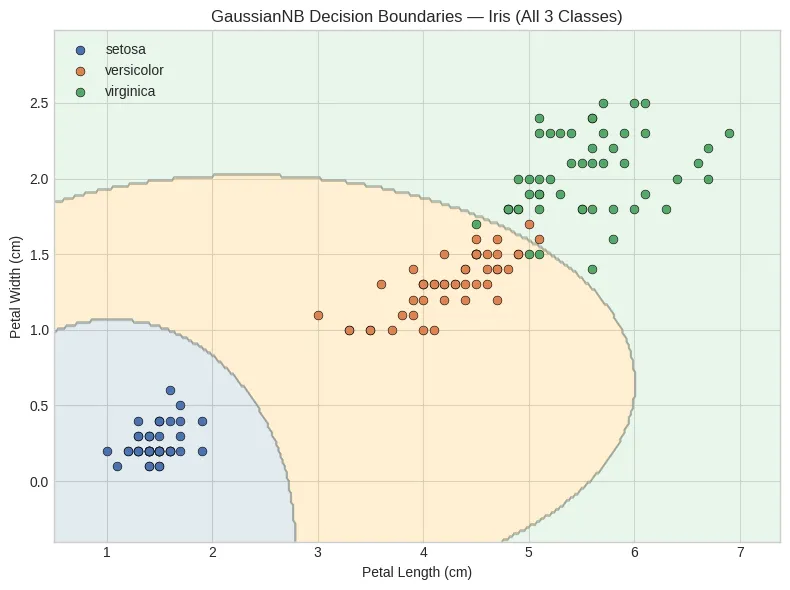 GaussianNB decision boundaries - Iris (petal length vs. petal width)
The posterior probability chart for a single test sample shows how confidently the model assigns probabilities. Even though the independence assumption is violated (petal length and petal width have 0.96 correlation), GaussianNB achieves 96% 5-fold cross-validation accuracy.
GaussianNB 5-fold CV Accuracy: 0.953 +/- 0.027
Individual fold scores: [0.933 0.967 0.933 0.933 1.   ]
MultinomialNB
For text classification, features are word counts - non-negative integers that fit the multinomial likelihood:
The Laplace smoothing parameter prevents the zero-frequency problem: if a word never appears in class 's training data, it would otherwise zero out the entire posterior. The notebook demonstrates this on the 20 Newsgroups dataset (4 categories: baseball, space, politics/guns, computer graphics):
vec = CountVectorizer(stop_words='english', max_features=10_000)
X_train_counts = vec.fit_transform(news_train.data)

mnb = MultinomialNB(alpha=1.0)
mnb.fit(X_train_counts, news_train.target)
Inspecting feature_log_prob_ reveals which words are most informative per category. The top words for sci.space include domain-specific terms like "nasa", "orbit", and "shuttle" - the model learns real linguistic signal, not noise.
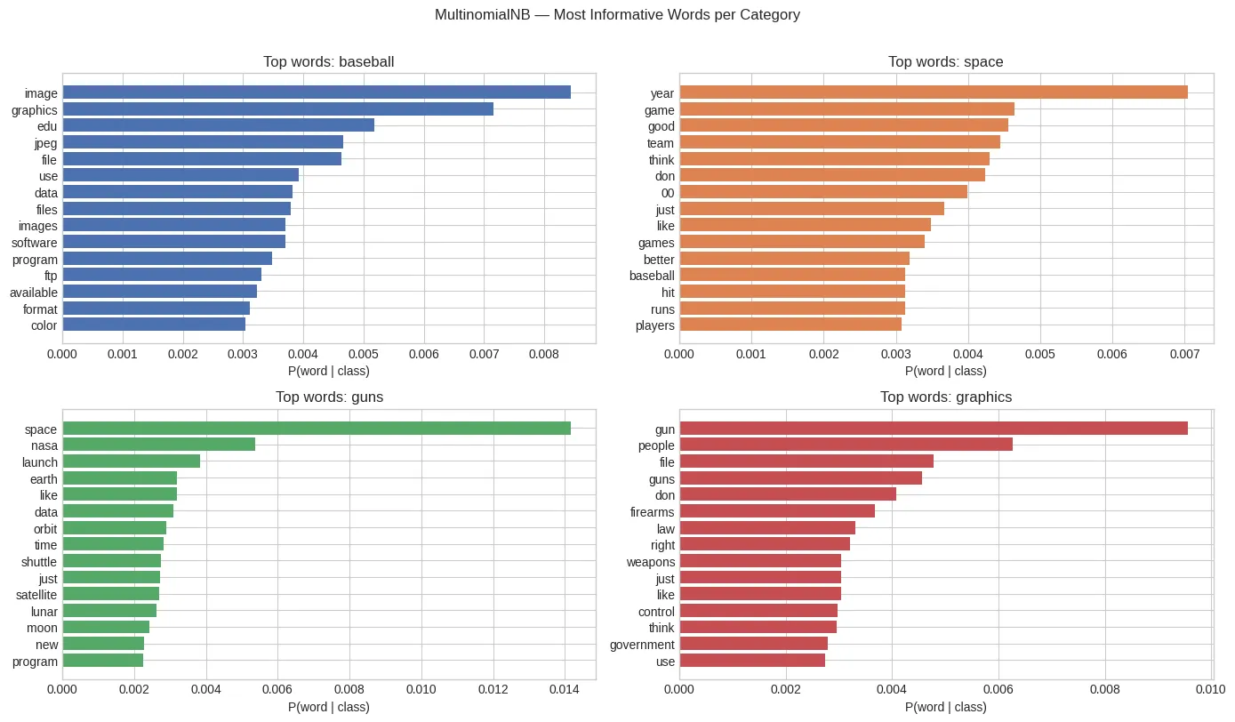 Most informative words per category - MultinomialNB on 20 Newsgroups
An alpha sweep shows how smoothing strength affects accuracy: too little smoothing (alpha near 0) causes overfitting on rare words; too much dilutes the signal. The optimal value is usually around 0.1–1.0.
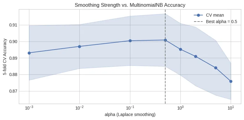 Laplace smoothing parameter sweep - 5-fold cross-validation accuracy
BernoulliNB
BernoulliNB treats each feature as a binary indicator: was this word present (1) or absent (0)?
The critical difference from MultinomialNB is the term - it penalizes the absence of a word. If "goal" is strongly associated with the sports class but absent from a document, BernoulliNB counts that as evidence against sports. MultinomialNB simply ignores absent words.
The notebook demonstrates this with a toy 5-word vocabulary: a document containing only "game" (ambiguous) is classified differently by the two models depending on whether their sports-class words are present.
| Model | Behavior for absent features | Best for |
|---|---|---|
| MultinomialNB | Ignores absent features | Long documents, articles |
| BernoulliNB | Penalizes absent features | Short texts, tweets, profiles |
On the 20 Newsgroups 4-category subset:
| Model | Test Accuracy | CV Accuracy (5-fold) |
|---|---|---|
| MultinomialNB | ~0.93 | ~0.92 |
| BernoulliNB | ~0.88 | ~0.88 |
MultinomialNB wins on longer documents (newsgroup posts average hundreds of words), but BernoulliNB can outperform on very short texts where frequency is uninformative.
Comparing All Three
| Property | GaussianNB | MultinomialNB | BernoulliNB | ComplementNB |
|---|---|---|---|---|
| Feature type | Continuous | Non-negative counts | Binary (0/1) | Non-negative counts |
| Likelihood | Gaussian PDF | Multinomial | Bernoulli | Complement multinomial |
| Penalizes absence? | N/A | No | Yes | No |
| Best for | Biology, sensors | Long text | Short text, profiles | Imbalanced text |
The independence assumption discussed in the Independent Events section is exactly what makes NB "naive" - and exactly why it still works: in classification, we only need the correct class to rank highest, not for probabilities to be exact.
SMS Spam Classifier
The notebook closes with the SMS Spam Collection - 5572 messages labeled ham or spam. The preprocessing pipeline mirrors the theoretical steps:
# 1. Clean - letters only, lowercase
text = re.sub('[^a-zA-Z]', ' ', text).lower().split()
# 2. Remove stopwords
text = [w for w in text if w not in stop_words]
# 3. Lemmatize
text = [lemmatizer.lemmatize(w, pos='v') for w in text]
# 4. TF-IDF vectorization
X = TfidfVectorizer(max_features=3000).fit_transform(corpus)
Four classifiers are then benchmarked on the same features:
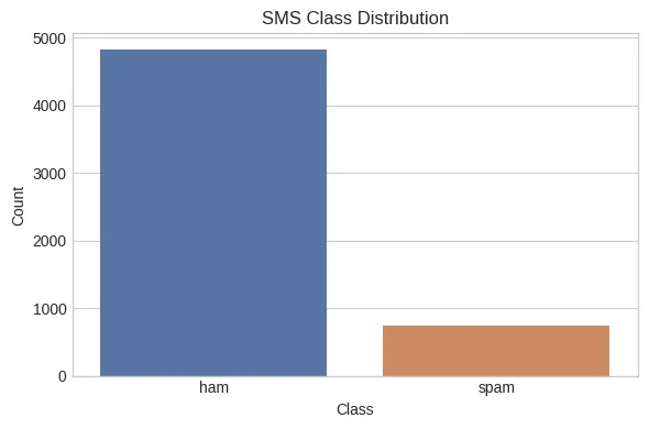 SMS dataset: heavily imbalanced toward ham ( 87% ham, 13% spam)
| Model | Precision | Recall | F1 | CV Accuracy (10x) |
|---|---|---|---|---|
| MultinomialNB | 0.97 | 0.94 | 0.95 | 0.97 |
| RandomForest | 0.98 | 0.94 | 0.96 | 0.97 |
| KNeighbors | 0.92 | 0.79 | 0.85 | 0.91 |
| SVC | 0.98 | 0.96 | 0.97 | 0.97 |
MultinomialNB performs competitively against Random Forest and SVC while requiring only a fraction of the training time. Its feature_log_prob_ parameters are directly interpretable, allowing inspection of which words contributed most to a spam prediction.
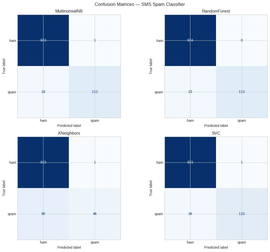 Confusion matrices: Random Forest achieves the best overall balance and produces no false positives, while MultinomialNB and SVC remain highly competitive. KNN performs substantially worse due to poor recall on the minority class.
Naive Bayes is the right baseline to beat before reaching for more complex models. It is fast, interpretable, and surprisingly competitive on text classification tasks-precisely the application where the “naive” independence assumption tends to be least harmful.
In the next article, we'll explore statistical tests and their role in machine learning.