Statistics and Machine Learning

We've already explored the workflow of a machine learning project and experimented with exploratory data analysis (EDA) and feature engineering (FE). Now, we'll delve a little deeper into some fundamental statistical concepts and see what we should consider when analyzing our data to ensure our models perform as well as possible.

Previous article in this series: Vectors and Machine Learning

Descriptive Statistics

Descriptive statistics is the branch of statistics that focuses on collecting, organizing, summarizing, and visualizing a dataset. Its main goal is to transform raw data into structured and understandable information, allowing us to understand "what happened" with the data we are analyzing.

We can divide its main tasks into 5 fundamental steps:

Collect: Obtain data from various sources, such as databases, CSV files, APIs, etc. This step is crucial to ensure we have a representative and high-quality sample for our analysis.
Organize: This involves organizing the collected information so we can analyze it: classifying variables or constructing frequency or distribution tables.
Present: Display the data clearly and in an organized manner, using tables, numerical summaries, or graphs. This facilitates the interpretation and communication of the results to others.
Summarize: Use numerical metrics to describe large volumes of data with a few key values. This is where measures of central tendency and dispersion come into play.
Interpret: Analyze the data and draw meaningful conclusions, using both numerical metrics and visualizations to communicate the findings effectively.

Variable Classification

The type of variable influences how we analyze data and what metrics we use:

Categorical Variables: Represent categories or groups. They can be:
Nominal: They do not have a specific order (colors, types of fruit).
Ordinal: They have an order or hierarchy (levels of satisfaction: low, medium, high).
Numerical Variables: Represent quantities or measurements. They can be:
Discrete: They take whole number values (number of children, number of cars).
Continuous: They can take any value within a range (height, weight, salary).

Frequency and Distribution Tables

Frequency tables are a fundamental tool for organizing and presenting categorical data. They allow us to count how many times each category occurs in our dataset, which facilitates the identification of patterns and trends. For example, if we have a variable "Car Color" with categories "Red," "Blue," and "Black," a frequency table would show us how many cars of each color are in our dataset.

Distribution tables, on the other hand, are used for numerical variables. They allow us to organize the data into intervals or ranges and count how many values fall within each interval. This is especially useful for understanding the shape of the data distribution, identifying skewness, or detecting outliers.

These types of tables (and graphs) allow us to detect issues such as skewed distributions, the presence of outliers, or the need to transform the data to improve the performance of our machine learning models.

Data Presentation

Data presentation is crucial for effectively communicating statistical findings. We can use:

Tables: To display information in a structured and detailed manner.
Charts: To visualize patterns, trends, and relationships in the data:
- Histograms: Show the distribution of a continuous variable.
- Box plots: Show the spread and the presence of outliers.
- Bar charts: Show comparisons between categories.
- Line charts: Show trends over time.

Statistical Measures

To summarize numerical data, two main families of metrics are used:

Measures of Central Tendency: These indicate where the data is clustered.
- Mean (Average): The sum of all values divided by the total number of data points. It is sensitive to extreme values (outliers).
  How do outliers affect it? If we have a dataset with atypical values, the mean can give us a misleading impression of the "center" of the data. For example, if most employees earn between $2,000 and $3,500, but there is an executive who earns $15,000, the mean will be higher, giving the false impression that the typical salary is much higher than it actually is for most people.
- Median: This is the central value of a dataset ordered from smallest to largest. It is robust and not easily misled by anomalies.
  How do you protect against outliers? The median gives us a better idea of the typical salary. In the previous example, if we have values like $2K, $2.2K, $2.5K, $2.5K, $2.8K, $3.1K, $3.5K, and an outlier of $15K, the median would be $2.65K, better reflecting the typical salary of most employees.
- Mode: The value (or values) that appears most frequently in the data set.
Measures of Dispersion: These provide information about the variability, or how spread out the data is.
- Range: The difference between the maximum and minimum values.
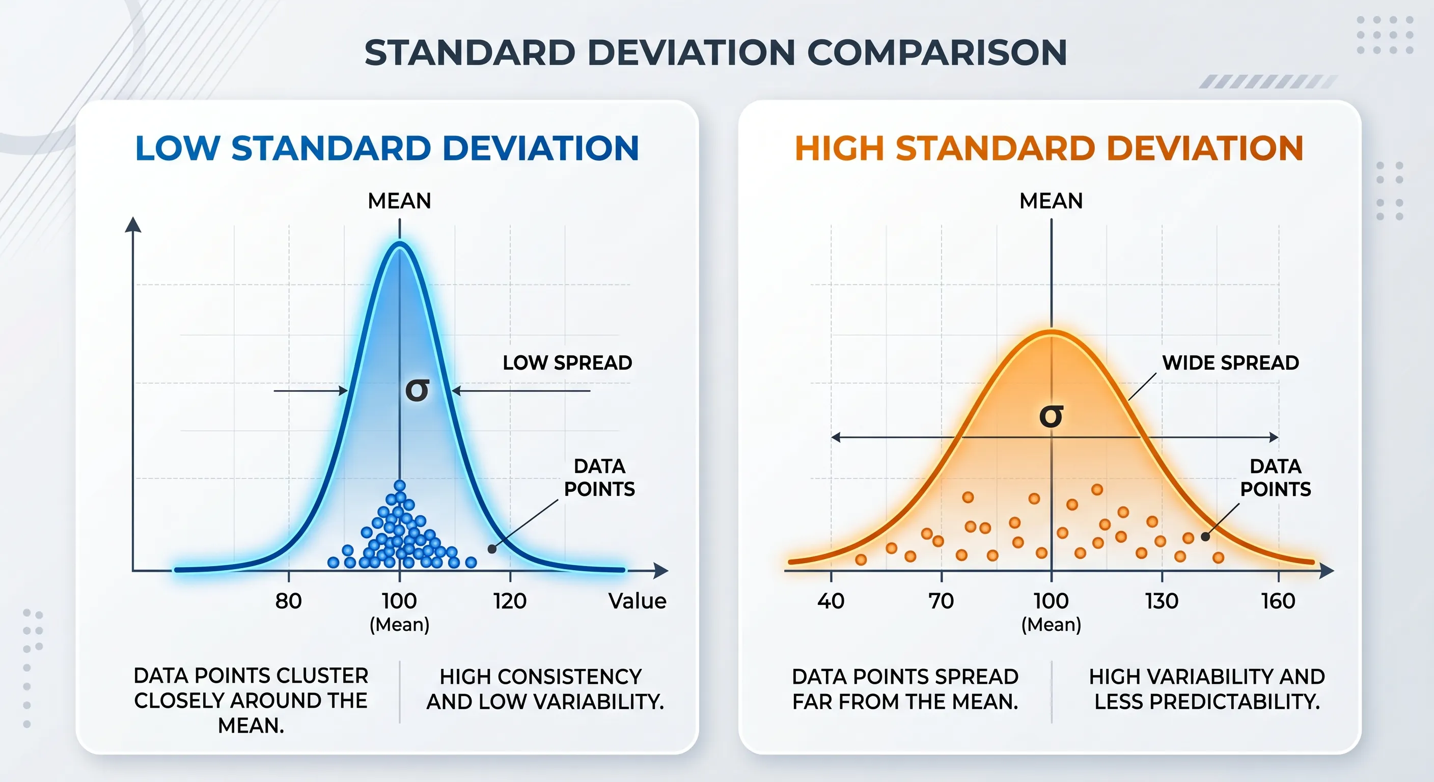
- Variance: Measures the average of the squared deviations from the mean.
  Why square? Because if we simply sum the deviations (values minus the mean), they will cancel each other out, resulting in zero. By squaring, all deviations become positive, allowing us to measure dispersion without the values canceling each other out.
- Standard Deviation: The square root of the variance. It is commonly used because it returns the measure to its original units.
- Interquartile Range (IQR): The difference between the 75th percentile (Q3) and the 25th percentile (Q1). It helps us understand the dispersion of the middle 50% of the data, ignoring outliers.
  Why is it useful? Because it allows us to understand the dispersion of most of the data without outliers distorting our perception. In the salary example, the IQR would show us the variability between the 25th and 75th percentiles of employees, providing a clearer view of the typical salary distribution.

How does a low or high standard deviation affect our machine learning models? A low standard deviation indicates that the data is tightly clustered around the mean, which can make it easier for models to learn clear patterns. On the other hand, a high standard deviation suggests that the data is more spread out, which can make it more difficult for models to find meaningful relationships and generalize well to new data.

Scatter plot with low and high standard deviation Let's see how to generate and analyze these statistics using pandas. Let's take the example of employee salaries:

import pandas as pd

# 1. Organizing the Data
# Most employees earn between $2,000 and $3,500, but one manager earns $15,000 (our outlier)
salaries = [2000, 2200, 2500, 2500, 2800, 3100, 3500, 15000]
df = pd.DataFrame({'Salary': salaries})

# 2. Measures of Central Tendency
mean = df['Salary'].mean()
median = df['Salary'].median()
mode = df['Salary'].mode()[0]

print("--- Central Tendency ---")
print(f"Mean: ${mean:.2f}")
print(f"Median: ${median:.2f}")
print(f"Mode: ${mode:.2f}\n")

# 3. Measures of Dispersion
range = df['Salary'].max() - df['Salary'].min()
variance = df['Salary'].var() # ddof=1 by default (sample)
std_dev = df['Salary'].std()
iqr = df['Salary'].quantile(0.75) - df['Salary'].quantile(0.25)

print("--- Measures of Dispersion ---")
print(f"Range: ${range:.2f}")
print(f"Variance: {variance:.2f}")
print(f"Standard Deviation: ${std_dev:.2f}")
print(f"IQR: ${iqr:.2f}")

Mean vs. Median: The mean is $4,200, inflated by the exaggerated $15,000. However, the median is **\$ 2,650**, much more representative of an average employee. When analyzing data, you should always check both for potential biases.
Mode: The most frequent salary level is $2,500.
Standard Deviation: We will obtain approximately $4,390.25. This is a huge dispersion caused again by the high salary being far removed from the others.
IQR: The Interquartile Range gives us $775, reaffirming that the "bulk" of the normal core of employees (the middle 50%) have salaries that vary within a much smaller and more manageable range.

A rule of thumb (but not an absolute one): If the mean is less than the median, then the distribution is left-skewed (negatively skewed). If the mean is greater than the median, then the distribution is right-skewed (positively skewed).

You can practice with other examples in the following Google Colab notebook.

Inferential Statistics

Another very important branch is inferential statistics. While descriptive statistics is limited to describing the data we have, inferential statistics allows us to draw conclusions about a population based on a sample. This is crucial in machine learning, since we often work with limited datasets and want to generalize our findings to a broader context.

Let's start by defining some key concepts:

Population

We will understand this as the entire set of individuals or elements that we want to study. For example, all the students at a university.

Sample

A subset of the population that is actually being studied. From all the students, we take 200 randomly selected.

Parameter

This is a numerical value that describes a characteristic of the population. We could, for example, take the average height of all the students.

Statistic

Unlike a parameter, a statistic is calculated from the sample. For example, we could have the mean height of 200 students.

Sampling Error

The difference between the true parameter and the estimated statistic. If the true mean height of the population is 1.70 m and the mean of our sample is 1.68 m, the sampling error would be 0.02 m. HOWEVER, in practice, we most likely won't know the true parameter, so the sampling error cannot be calculated directly. Instead, the standard error is usually calculated, which is an estimate of the variability of the statistic due to random sampling. The standard error is calculated as:

SE = \frac{\sigma}{\sqrt{n}}

Where $\sigma$ is the population standard deviation (or an estimate based on the sample) and $n$ is the sample size.

Confidence Level

The probability that an estimate contains the true parameter. If we say we have a 95% confidence interval, it means that if we repeated the sampling process many times, approximately 95% of those intervals would include the true population parameter. It is a measure of how confident we are in our estimates.

Confidence Interval

A confidence interval (CI) is a range of values within which the population parameter is expected to lie with a certain level of confidence. In simple terms, it is a way of expressing the uncertainty of our estimates. For example, if we calculate a 95% confidence interval for the mean height of the students and obtain (1.65m, 1.75m), we can say that we are 95% confident that the true mean height of all students lies between these two values.

Basic formula:

IC = \bar{x} \pm Z \left(\frac{\sigma}{\sqrt{n}}\right)

Where:

$\bar{x}$ = sample mean
$Z$ = critical value
$\sigma$ = standard deviation
$n$ = sample size

This formula is used to calculate the confidence interval for the population mean when the standard deviation is known and the sample size is sufficiently large (n > 30).

In practice, we often don't know the population standard deviation, so we use the sample standard deviation and the critical value of the Student's t-distribution instead of Z. The formula is:

CI = \bar{x} \pm t \left(\frac{s}{\sqrt{n}}\right)

Where:

$\bar{x}$ = sample mean
$t$ = critical value of the Student's t-distribution
$s$ = sample standard deviation
$n$ = sample size

With that clarified, let's look at a practical example:

A survey of 100 people reveals that the average monthly expenditure is $50, with a standard deviation of $10 and a 95% confidence level.

We know that:

Z = 1.96

For a 95% confidence level, the critical Z-value is approximately 1.96 (this is obtained from the standard normal distribution table).

You can find out more about how to obtain this value by researching the standard normal distribution and Z-tables (I hope to publish an article about this soon).

We calculate:

IC = 50 \pm 1.96 \left(\frac{10}{\sqrt{100}}\right)

IC = 50 \pm 1.96 (1)

IC = 50 \pm 1.96

Result:

IC = (48.04 , 51.96)

Interpretation: With 95% confidence, the true average population expenditure is between $48.04 and $51.96.

Hypothesis Testing

These tests are used to make decisions about a claim regarding a population. Let's break it down:

Basic Components

Null Hypothesis ( $H_0$ )

A claim we are testing, generally a claim of "no difference," "no effect," or "equality." Example: "The mean is equal to 50."

Alternative Hypothesis ( $H_1$ )

This represents the claim for which we are seeking evidence. It is the opposite of the null hypothesis. For example: "The mean is different from 50."

Significance Level ( $α$ )

This is the probability of rejecting $H_0$ when it is true. In other words, the risk we are willing to take of committing a Type I error (false positive). Values such as 0.05 (5%), 0.01 (1%), or 0.10 (10%) are commonly used as significance levels.

Test Statistic

The calculated value used to decide whether to reject $H_0$ .

p-Value

The probability of obtaining a result as extreme as the observed one if $H_0$ were true. If the p-value is less than $\alpha$ , we reject $H_0$ ; otherwise, we do not reject $H_0$ .

The p-value tells us how likely it is to obtain the results we have (or more extreme results) if the null hypothesis were true. If this probability is very low (less than our significance level), then we have sufficient evidence to reject the null hypothesis. For example, if we obtain a p-value of 0.03 and our significance level is 0.05, this means there is only a 3% probability of obtaining those results if the null hypothesis were true, leading us to reject H0.

Let's look at a practical example:

A company claims that the average delivery time is 30 minutes.

A sample is taken and the following is obtained:

n = 36
mean = 32 minutes
standard deviation = 6
$\alpha$ = 0.05

We formulate hypotheses

H_0: \mu = 30

H_1: \mu \neq 30

We calculate the Z statistic

Z = \frac{\bar{x} - \mu}{\sigma/\sqrt{n}}

Where:

$\bar{x}$ = sample mean = 32
$\mu$ = hypothesized mean = 30
$\sigma$ = standard deviation = 6
$n$ = sample size = 36

Z = \frac{32 - 30}{6/\sqrt{36}}

Z = \frac{2}{1}

Z = 2

Obtain the p-value:

For Z = 2, the p-value is approximately 0.0455 (using a standard normal distribution table or a statistical calculator).

Compare with $\alpha$ :

Since 0.0455 < 0.05, we conclude that:

$H_0$ is rejected

Now let's explain in more detail how to interpret this result and the steps we have taken:

First of all, let's understand something about this exercise: we have a population in which the average delivery time is unknown, but the company claims it is 30 minutes. We then take a sample of 36 deliveries and obtain a mean of 32 minutes with a standard deviation of 6 minutes. We want to calculate how compatible this sample mean of 32 minutes is with the claim that the population average time is 30 minutes.

The formula for obtaining Z standardizes the difference between the sample mean (32 minutes, OUR OBSERVATION) and the hypothesized mean (30 minutes, THE COMPANY'S CLAIM) in terms of standard deviations.

The calculated Z-value of 2 indicates that the sample mean is 2 standard deviations above the hypothetical mean of 30 minutes. In other words, if the average delivery time were truly 30 minutes, obtaining a sample mean of 32 minutes (as is the case here) would be a result 2 standard deviations higher than expected.

When working with a standard normal distribution, approximately 95% of the values are between -1.96 and 1.96, and 5% are outside that range (2.5% in each tail). Therefore, if we assume that $H_0$ is true, we would expect the sample mean to typically fall close to 30 minutes. However, obtaining a Z-value of 2 implies that with this value of 32 minutes, we are in a range that occurs approximately 4.55% of the time (two-tailed p-value), which is less than our significance level of 5%.

In other words, if the actual average were 30 minutes, only in 4.55% of the samples could we obtain a difference equal to or greater than 32 minutes by pure chance. That is, those 32 minutes would be very rare if the average time were truly 30 minutes.

A hypothesis test doesn't actually tell us whether $H_0$ is true or false. We are NOT saying that the delivery time is definitely different from 30 minutes, but rather that there is statistically significant evidence to conclude that the average delivery time is different from 30 minutes.

The formal conclusion would be:

With a significance level of 5%, the observed data are sufficiently incompatible with the claim that the average delivery time is 30 minutes, therefore we reject the null hypothesis.

As an aside:

Another equivalent way to analyze the problem is by using a 95% confidence interval for the population mean.

The formula for the interval is:

IC = \bar{x} \pm Z \left(\frac{\sigma}{\sqrt{n}}\right)

We know that $\bar{x} = 32$ , $Z = 1.96$ , $\sigma = 6$ and $n = 36$ .

IC = 32 \pm 1.96 \left(\frac{6}{\sqrt{36}}\right)

IC = 32 \pm 1.96 (1)

IC = (30.04 , 33.96)

The value 30 is NOT within the confidence interval

This means that, with 95% confidence, the true average is not 30 minutes.

Rejecting $H_0$ at the 5% level is exactly equivalent to the hypothesized value (30) falling outside the 95% confidence interval.

Two-tailed tests and confidence intervals tell the same story, just from different perspectives.

Returning to the previous conclusion:

It's not the same to say: "It's unlikely that the average delivery time is 30 minutes."

The classic test doesn't calculate:

$P(H_0 | data)$ - that is, the probability that $H_0$ is true given the data we have.

Instead, it calculates:

$P(data|H_0)$ - the probability of obtaining the data we have (or more extreme values) assuming that $H_0$ is true.

And it's also important to be clear on these three points:

That not rejecting $H_0$ is not the same as accepting $H_0$ . If the p-value had been greater than 0.05, we simply wouldn't have enough evidence to reject $H_0$ , but that doesn't mean that $H_0$ is true; it simply means that the data don't allow us to conclude that it's false. Remember that we are working with a sample.
That there is no absolute certainty. In this case, there is a 4.55% probability of committing a Type I error (rejecting H0 when it is true).

And there is also the possibility that the difference is statistically significant but has no practical relevance (that is, that the 2-minute difference is not important in reality).

Another interesting aspect we can analyze is the effect size. The difference we have is 2 minutes, but the standard error is 1 minute (this is the sigma/sqrt{n}$ part of the Z calculation). This makes the difference "large" in statistical terms, but if the sample had been only 9 people, the standard error would be 2 minutes, and the Z would be 1, which would not give us enough evidence to reject H0.

Significance depends on the sample size. A small difference can be significant if the sample is large.

About the Types of Errors

Type I Error (False Positive) Rejecting $H_0$ when it is true. For example, concluding that the delivery time is different from 30 minutes when it actually is.
Type II Error (False Negative) Not rejecting $H_0$ when it is false. For example, concluding that the delivery time is equal to 30 minutes when it is actually different.

Importance in Machine Learning

In machine learning, it is not enough to compare metrics and choose the model with the highest value. The metrics we obtain (accuracy, precision, recall, AUC, etc.) are sample estimates of the model's actual performance.

That is:

The dataset we use is a sample of the real world.
The calculated metric is a statistic.
The actual performance in production is an unknown population parameter.

Therefore, all comparisons between models are subject to sampling variability. If we took a different sample from the same problem, the metrics would change.

Here, the same problem we saw earlier arises:

Is the observed difference real, or can it be explained by chance?

Suppose we compare two binary classification models on a test set of 1000 observations:

Model A: accuracy = 0.85
Model B: accuracy = 0.80

The difference is 5%, but is this difference statistically significant? Is Model A really better than Model B, or could this difference be due to chance?

We could, for example, construct a confidence interval for the accuracy, allowing us to estimate a plausible range for the model's actual performance.

Another case would be comparing two models on the same test set (as is commonly done), which introduces dependence between the observations. This is important to consider because:

We cannot use tests for independent samples.
We need tests for paired data.

Some common tools include:

McNemar's test: for comparing accuracy in binary classification.
Paired t-test: when using cross-validation and obtaining multiple measurements.
Bootstrap: for estimating the empirical distribution of the difference between models.